Kulback Leibler Divergence

Introduction

To measure the difference between two probability distributions over the same variable $x$, a measure, called the Kullback-Leibler divergence (also known as the relative entropy) is used. Before we get into the formal notation, lets understand divergence itself.

Divergence vs Distance

More often than not we have single random variable and two different probability distributions to compare. Quantifying the difference between the distributions is of top importance expecially in machine learning. This problem is referred to as the problem of calculating the statistical distance between two statistical objects, e.g. probability distributions.

One approach is to calculate a distance measure between the two distributions. This can be challenging as it can be difficult to interpret the measure.

Although the KL divergence measures the distance between two distributions, it is not a distance measure. This is because that the KL divergence is not a metric measure and is non-symmetric.

Non-Symmetric

Divergence is a scoring of how one distribution differs from another, where calculating the divergence for distributions $p(x)$ and $q(x)$ would give a different score from $q(x)$ and $p(x)$. Thus the KL from $p(x)$ to $q(x)$ is not the same as $q(x)$ to $p(x)$.

Formally we write KL divergence as below.

The KL divergence is non-symmetric between two probability distributions $p(x)$ and $q(x)$ denoted as,

\begin{equation} D_{KL}(p(x)\vert \vert q(x)) \end{equation}

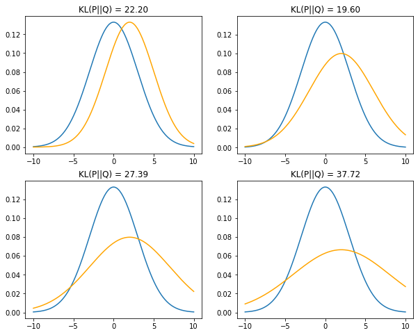
The divergence is used to measure the information loss when $q(x)$ is used to approximate $p(x)$. Formally it can be written as,

\begin{equation} D_{KL}(p(x)\vert \vert q(x)) = \sum_{x \in X}p(x) log(\frac{p(x)}{q(x)}) \end{equation}

Typically $p(x)$ represents the true distribution of data or a precisely calculated theoretical distribution. The measure $q(x)$ typically represents a theory, model, description, or approximation of $p(x)$.

Observations

Let’s make some observations from the above equation.

1. The KL divergence of a distribution with itself is zero, because $log(\frac{p(x)}{p(x)})$ = $log(1)$ = 0.
2. KL divergence between two distributions is always non-negative. We can show this with Jensen’s inequality. (We wont go into the proof here)

Jensen’s inequality: tells us that, the line connecting two points on a convex curve lies above the curve itself, and the expectation of a convex function is greater than the convex function of the expectation.

1. Another important thing to note here is that, KL’s lack of symmetry means that it fails to meet the definition of a metric (because when we say distance, metrics closely match out intution of a “distance” between two objects.)

Applications of divergence.

A typical application of divergence is approximating a target probability distribution when optimizing a Generative Adversarial Networks (GAN’s). Here is a nice explanation of GAN’s and minimizing divergence.

---

Python Implementation

The below implementation in Python. The function retutns the divergence score between two normal distributions.

def kl_divergence(p, q):
    prob = np.sum(np.where(p != 0, p * np.log(p / q), 0))
    return prob

Figure 1: Kl Divergence