Randomised approach to matrix decomposition: Fast SVD
We will cover the following topics in this post.
- Introduction to SVD
- Decomposing the Matrix
- SVD Properties
- Python implementation
- SVD vs Fast-Ramdomised-SVD
- Why use Randomized Matrix Approximation
- Fast SVD Method
- Resources
Introduction
“SVD is not nearly as famous as it should be.” - Gilbert Strang
When we think about dimentionality reduction and in particular matrix decomposition “PCA” and “Singular Value decomposition” is what comes to mind. In this post we will dive deeper into its computations and parallelly apply in it to a text dataset.
The SVD algorithm factorizes a matrix into one matrix with orthogonal columns and one with orthogonal rows (along with a diagonal matrix, which contains the relative importance of each factor).
SVD can be simply written as;
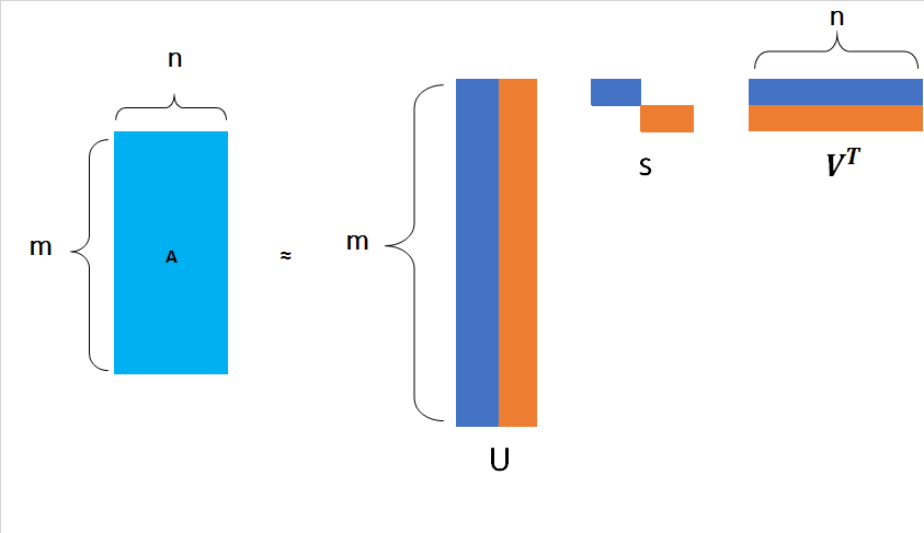
\begin{equation} A_{[m \times n]} = U_{[m \times r]} S_{[r \times r]} (V_{[n \times r]}) \end{equation}
Let’s look at each element of the above matrix decomposition.
- $A$ : Input Data matrix. $[m \times n]$ : eg. $m$ movies and $n$ users. (See example below)
We can think about it as an the input as a Matrix $A$ is of size $m \times n$, which means it has $m$ rows and $n$ columns. This matrix $A$ can be thought of as a Document Matrix with $m$ documents and $n$ terms in it. That means every row reprements a document and every column reprements a word in it.
Every document is represented as on long vector with $0$ and $1$ meaning the given word appears or does not appear in the document. We will see this in the below newsgroup dataset.
Alternatively consider the matrix as a movie user matrix such that every row as a different user and every column as a different movie.
The Decomposition
The idea is to take the matrix $A$ and represent it as product of 3 matrices, $u$, $s$ and $v$. This idea of taking the original matrix and representating it as a product of three different matrices is singular value decomposition. Specifically the matrix has few properties.
-
$U$ : Left Singular vectors. $[m \times r]$ ($m$ movies and $r$ concepts) . We can think of $r$ concepts as a very small number. We will come back to this later.
-
$S$: Singular values. $[r \times r]$ diagonal matrix. It basically represents the strength of the matrix $A$. Here we have only non-zero elements across the diagonal which we call as singular values. The singlular values are sorted in the decreasing order.
-
$V$: Right Singular values. $[n \times r]$ matrix where $n$ is the number of columns from the original matrix and $r$ we can think of as a small number basically the rank of the matrix $A$.
We can pictorically represent this as below.
SVD Properties
The “SVD” theorem says that “It is always possible to decompose a real matrix $A$ into $A = USV^T$ where,
- $U$, $S$, $V$ are unique.
- $U$ and $V$ are column orthonomal i.e $U^T U = I$, $V^T V = I$ $I$ : Identity matrix.
- $S$ Entries in the singular values are positive and sorted in descreasing order.
Implementation
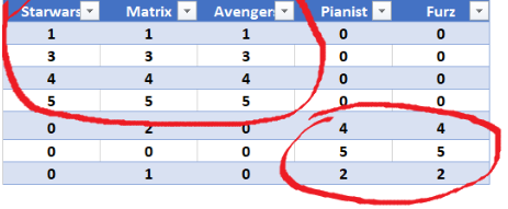
Consider the Matrix user to movie.
Lets think of this example as a movie review website. Here each row represents user and the column represents different movie. 1 Being the lowest and 5 being the higest rating.
So a user say no.3 likes more of Scify moves as compared to War movies, hence the column 4 and 5 are 0.
Our goal here is to deompose this matrix into three components. Visually we can see that the users can be broken down into two groups as seen below.
Let’s demonstrate this with the standard scipy object linalg where svd is defined.
from sklearn.datasets import fetch_20newsgroups
from scipy import linalg
import numpy as np

a= np.matrix('1 1 1 0 0; 3 3 3 0 0; 4 4 4 0 0 ; 5 5 5 0 0; 0 2 0 4 4; 0 0 0 5 5; 0 1 0 2 2')
a

matrix([[1, 1, 1, 0, 0],
        [3, 3, 3, 0, 0],
        [4, 4, 4, 0, 0],
        [5, 5, 5, 0, 0],
        [0, 2, 0, 4, 4],
        [0, 0, 0, 5, 5],
        [0, 1, 0, 2, 2]])

> print("Shape of original matrix:" , a.shape)
Shape of original matrix: (7, 5)

> U, s, v = linalg.svd(a, full_matrices=False)
Strength of the scifi concept. Here we see that the strength of the scify concept is more than the “War movie” concept.
Take a look at the diagonal matrix.
> np.round(np.diag(s), 3)

array([[12.481,  0.   ,  0.   ,  0.   ,  0.   ],
       [ 0.   ,  9.509,  0.   ,  0.   ,  0.   ],
       [ 0.   ,  0.   ,  1.346,  0.   ,  0.   ],
       [ 0.   ,  0.   ,  0.   ,  0.   ,  0.   ],
       [ 0.   ,  0.   ,  0.   ,  0.   ,  0.   ]])
User to concept matrix.
Matix $U$ we see that the first four users belong to more of SciFy concepy.
array([[-0.14, -0.02, -0.01,  0.56, -0.38],
       [-0.41, -0.07, -0.03,  0.21,  0.76],
       [-0.55, -0.09, -0.04, -0.72, -0.18],
       [-0.69, -0.12, -0.05,  0.34, -0.23],
       [-0.15,  0.59,  0.65,  0.  ,  0.2 ],
       [-0.07,  0.73, -0.68,  0.  ,  0.  ],
       [-0.08,  0.3 ,  0.33,  0.  , -0.4 ]])
Matrix $V$ we can relate to as a “movie-to-concept” matrix as the first three refers to more of the first concept (scifi) whereas the last 2 (0.69) relate to “war movie” concept.
In both cases we see we see the third concept which is more or less modelled as “noise” in our data.
> np.round(v, 3)

array([[-0.56, -0.59, -0.56, -0.09, -0.09],
       [-0.13,  0.03, -0.13,  0.69,  0.69],
       [-0.41,  0.81, -0.41, -0.09, -0.09],
       [-0.71,  0.  ,  0.71,  0.  ,  0.  ],
       [ 0.  , -0.  ,  0.  , -0.71,  0.71]])
SVD vs Fast Ramdomised SVD
The good thing about SVD is that we have a method that allows us to exactly factor a matrix into orthogonal columns and orthogonal rows. Lets demonstrate this in our news group dataset inbuilt in sklearn
Newsgroups are discussion groups, which was popular in the 80s and 90s. This dataset includes 18,000 newsgroups posts with 20 different topics. We would like to find topics which are Orthogonal.
Now our idea is that, We would clearly expect that the words that appear most frequently in one topic would appear less frequently in the other - otherwise that word wouldn’t make a good choice to separate out the two topics. Therefore, we expect the topics to be orthogonal.
from sklearn.datasets import fetch_20newsgroups
from sklearn.feature_extraction.text import CountVectorizer
from sklearn import decomposition
import fbpca

categories = ['alt.atheism', 'talk.religion.misc', 'comp.graphics', 'sci.space']
remove = ('headers', 'footers', 'quotes')
newsgroups_train = fetch_20newsgroups(subset='train', categories=categories, remove=remove)
newsgroups_test = fetch_20newsgroups(subset='test', categories=categories, remove=remove)

vectorizer = CountVectorizer(stop_words='english')
vectors = vectorizer.fit_transform(newsgroups_train.data).todense()
> %time u, s, v = np.linalg.svd(vectors, full_matrices=False)

Wall time: 39.6 s
> %time u, s, v = decomposition.randomized_svd(vectors, n_components=10)

Wall time: 23.4 s
# using facebook's pca
> %time u, s, v = fbpca.pca(vectors, 10)

Wall time: 3.48 s
Clearly the Randomes approach to SVD is much faster. Lets discuss the method and its implementation.
Randomized Matrix Approximation
Need for a Randomized Approach
Matrix decomposition remains a fundamental approach in many machine learning tasks especially with the advent of NLP. With the development of new applications in the field of Deep learning, the classical algorithms are inadequate to tackle huge tasks. Why?
-
Matrices are enormously big. Classical algorithms are not always well adapted to solve the type of large-scale problems that now arise in Deep learning.
-
More often than not Data are missing. Traditional algorithms which produce accurate Matrix decomposition but ends up in using extra computational resources.
-
Passes over data needs to be faster, since data transfter plays an important role. For this GPU’s can be effectively utilized.
Method
Randomised approach to matrix decomposition was discussed in the paper, Finding Structure with Randomness: Probabilistic Algorithms for Constructing Approximate Matrix Decompositions by Nathan Halko, Per-Gunnar Martinsson and Joel A. Tropp and later summarized by Facebook in this blog post. The method was proposed for general purpose algorithms used for various matrix approximation tasks.
Idea: Use a smaller matrix (with smaller $n$)!
Instead of calculating the SVD on our full matrix $A$ which is $[m \times n]$, we use $B = AQ$, which is a $[m \times r]$ matrix where $r « n$.
Note: This is just a method with a smaller matrix!!
1. Compute an approximation to the range of $A$. That is, we want $Q$ with $r$ orthonormal columns such that $A \approx QQ^TA$. See randomized_range_finder() below.
2. Construct $B = Q^T A$, which is small ($r\times n$)
3. Compute the SVD of $B$ by standard methods i.e $B = S\,\Sigma V^T$. This is fast since $B$ is smaller than $A$.
4. Substituting back to $A$ we have,
\[A \approx Q Q^T A \\\] \[= Q (S\,\Sigma V^T) \space \text{as} \space B = Q^T A \\\] \[= U \Sigma V^T \space \text{if we construct} \space U = QS\]We now have a low rank approximation $A \approx U \Sigma V^T$.
Trick in finding $Q$
To estimate the range of $A$, we can just take a bunch of random vectors $\omega_i$, evaluate the subspace formed by $A\omega_i$. We can form a matrix $\Omega$ with the $\omega_i$ as it’s columns.
Now, we take the QR decomposition of $A\Omega = QR$, then the columns of $Q$ form an orthonormal basis for $A\Omega$, which is the range of $A$.
Since the matrix $A\Omega$ of the product has far more rows than columns and therefore, approximately, orthonormal columns. This is simple probability - with lots of rows, and few columns, it’s unlikely that the columns are linearly dependent.
Lets do this in Python. The method below randomized_range_finder finds an orthonormal matrix whose range approximates the range of $A$ (discussed in step 1 above). This is done using the scikit-learn.extmath.randomized_svd source code.
def randomized_range_finder(A, size, n_iter=5):
    Q = np.random.normal(size=(A.shape[1], size))

    for i in range(n_iter):
        # compute the LU decomposition of the matrix
        Q, _ = linalg.lu(A @ Q, permute_l=True)
        Q, _ = linalg.lu(A.T @ Q, permute_l=True)

    # QR decomposition
    Q, _ = linalg.qr(A @ Q, mode='economic')
    return Q

def randomized_svd(M, n_components, n_oversamples=10, n_iter=4):

    n_random = n_components + n_oversamples

    Q = randomized_range_finder(M, n_random, n_iter)

    # project M to the (k + p) dimensional space using the basis vectors
    B = Q.T @ M

    # compute the SVD on the thin matrix: (k + p) wide
    Uhat, s, V = linalg.svd(B, full_matrices=False)
    del B
    U = Q @ Uhat

    return U[:, :n_components], s[:n_components], V[:n_components, :]
> %time u, s, v = randomized_svd(vectors, n_components=10)

Wall time: 11.1 s
Resources
You can find the whole notebook for this at my GitHub.
[1] Finding Structure with Randomness: Probabilistic Algorithms for Constructing Approximate Matrix Decompositions is an excellent read.
[2] FastAI Numerical Linear Algebra.