Dealing with an unbalanced dataset
During my recent project i came accross this problem where all the predictions where biased towards one particular class. The problem was quite obvious pointing to my unbalanced data. Here is an illustration.
What are Unbalanced data ?
Unbalanced data as the name suggests, refers to the situations where we have unequal instances of classes/target variables. While implementing a classification algorithm, i frequently come accross this problem. Some examples of such an unbalanced class can be quite often seen in a cancer data set where one has twice the number of benign cases as compared to malignant class. Or when building an object detector for a vechicle, we quite commonly come across more no of non-cars images as compared to cars in our data set.
Let’s look at a such a dataset, UCI Breast cancer Dataset which we can use to for our study here.
An example of such an unbalanced class can be seen here.
rm(list = ls())
library(caret)
# read data
df <- read.table("Data/breast-cancer-wisconsin.txt", header = FALSE,  sep = ",")

# update column names
colnames(df) <- c("sample_no", "clump_thickness", "cell_size", "cell_shape",
                "marginal_adhesion","single_epithelial_cell_size",
                "bare_nuclei", "bland_chromatin", "normal_nucleoli",
                "mitosis", "classes")

# update the classes
df$classes <- ifelse(df$classes == "2", "benign", ifelse(df$classes == "4", "malignant", NA))
A quick plot between two features can be shown to visualize the class imbalances.
ggplot(data = df, aes(x=df$cell_size, y=df$cell_shape, color=classes))+
    geom_point(size=2)+
    labs(x='Cell Size', y='Cell Shape')+
    theme(panel.grid.major = element_blank(), panel.grid.minor = element_blank())
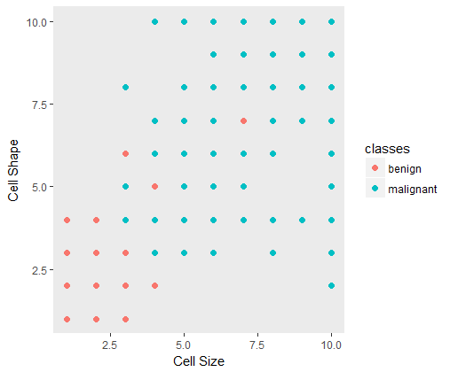
Looking at the class labels in the data set shows the imbalance in both the classes.
# A look at our class labels

> table(df$classes)
   benign malignant
      458       241
Why this problem needs to be addressed ?
Most classification algorithms are sensitive to the the predictors i.e the class labels. Consider the above case where benign cases are 458 which is almost double the number of malignant cases. The algorithm once trained will be more biased towards the benign cases and predict most of the test cases as benign and thus wont generalize well.
Also important to consider that, in such a case, the algorithm will generate a high accuracy since the benign cases are more, which is of-course misleading.
Pitfalls of Up-sampling and Down-sampling.
Traditionally one can always up-sample or down-sample the data. In practise this is not really advisible since it could lead to inappropriate cross-validation scores.
Over-sampling by replication can lead to similar but more specific regions in the feature space as the decision region for the minority class. This can potentially lead to overfitting on the multiple copies of minority class samples.
SMOTE Sampling Technique
SMOTE was developed to generate synthetic examples by operating on the feature space.
The minority class is over-sampled by taking each minority class sample and introducing synthetic examples along the line segments joining any or all of the k minority class nearest neighbors. Depending upon the amount of over-sampling required, neighbors from the k nearest neighbors are randomly chosen.
Generating Synthetic samples take the following way:
- Take the difference between the sample (the feature vector) and its nearest neighbor.
- Multiply the difference by a random number between 0 and 1 and add this to the feature vector (i.e the sample point under consideration.)
In effect what this does is that a random point is reinstated along the line segment between two specific features.
This can be conviniently performed in R using the SMOTE() function we call from the library(DMwR).
# split data into train and test
dfindex <- createDataPartition(df$classes, p = 0.7, list = FALSE)
train_data <- df[dfindex, ]
test_data  <- df[-dfindex, ]
Lets look at the original labels in training set.
> table(train_data$classes)

   benign malignant
      321       169
Using SMOTE(), we can oversample the minority class. The function takes the parameter perc.over which over samples. perc.under paramater can also be used to undersample the majority class. A typical example is below,
library(DMwR)
dat <-  SMOTE(classes~., data = train_data[c(2:11)], perc.over = 100, k = 3)

> table(smote_train$classes)

   benign malignant
      338       338
Codes for this post is on my GitHub. A nice explanation about SMOTE is here