Rectified ADAM Optimizer
Introduction
The buzzword among the Deep Learning community is about the latest revision to Optimization algorithm ADAM published by Liyuan Liu known as the Variance of Adaptive Learning, Rectified Adam.
In this post we first talk about the difference and why the authors claim that R-Adam works better. Subsequently we implement this on CIFAR-10 using Keras. Note i am using the revised Tensorflow 2.0 backed Keras, so you might have to tweak the code if you are on the older verion Tensorflow 1.14.
So let’s directly dive into it. Here is what we cover.
Adaptive Learning
We know the problem of setting different learning rates during training with SGD. Choosing the learning rate turns out to be a difficult hyper-parameter to set during training a network. The learning rate also significantly effects the model performance. SGD with momentum algorithm in a way address this problem, but it only comes with the cost of adding another hyperparameter. It thus made sense to use a separate learning rate for each parameter and automatically adapt it during the training phase. This led to the development of algorithms with the so called adaptive learning rates. These can be studied as a family of three algorithms which are simple modifications of one another namely, ‘AdaGrad’, ‘RMSProp’, ‘Adam’.
Recall that,
‘Adagrad’ maintains a per-parameter learning rate that improves performance on problems with sparse gradients.
‘RMSProp’ also maintains per-parameter learning rates that are adapted based on the average of recent magnitudes of the gradients for the weight (e.g. how quickly it is changing).
ADAM
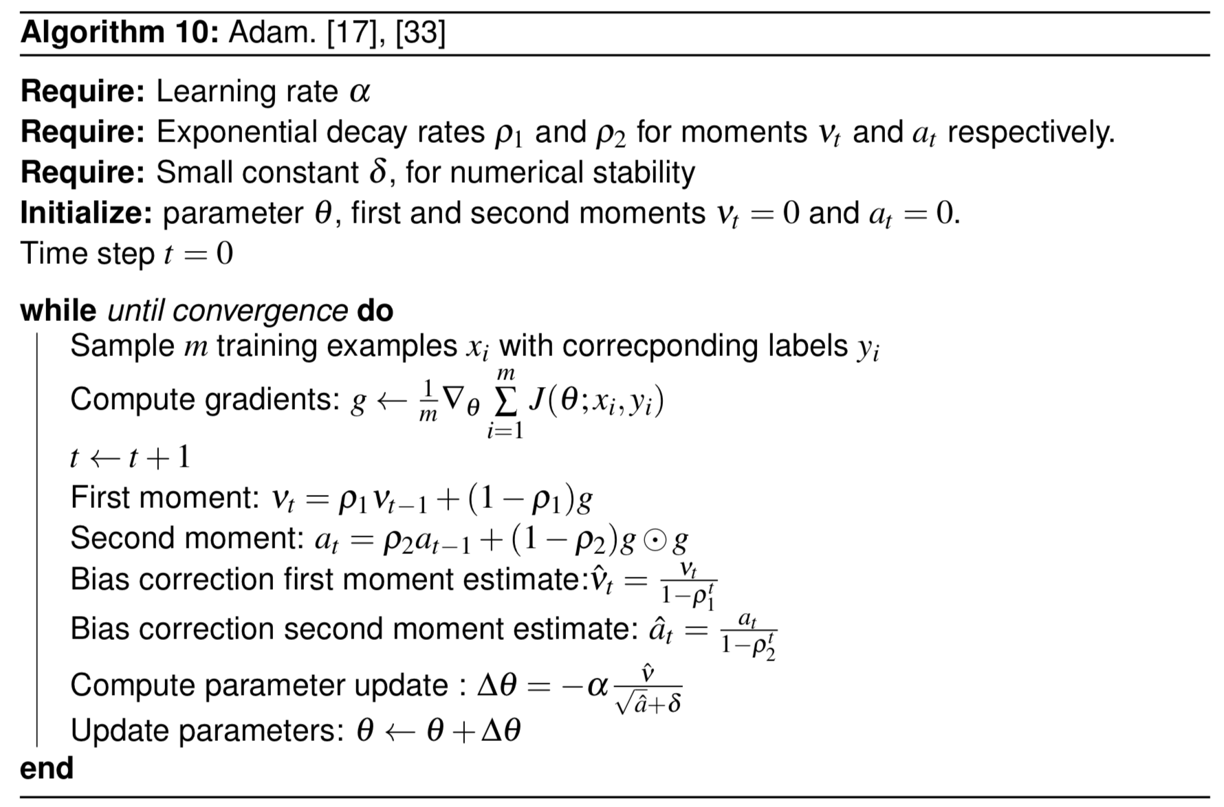
“Adam” as the name goes derives from the concept of “adaptive moments”. It applies the best of the both world’s, meaning, a combination of two methods ‘RMSProp’ and ‘AdaGrad. The method computes individual adaptive learning rates for different parameters from estimates of first and second moments of the gradients. It can be described in two steps.
First: Add momentum to RMSprop, which means adding momentum to rescaled gradients. It does this by computing the moments. The algorithm calculates an exponential moving average of the gradient and the squared gradient. The two parameters rho1 and rho2 control the decay rates of these moving averages.
Second: It was observed that the moment estimnates are biased towards 0, especially when the decay rates are small (or close to 1). These biases are corrected by computing the first and second moment estimates.
The algorithm is summarised below.

R-Adam
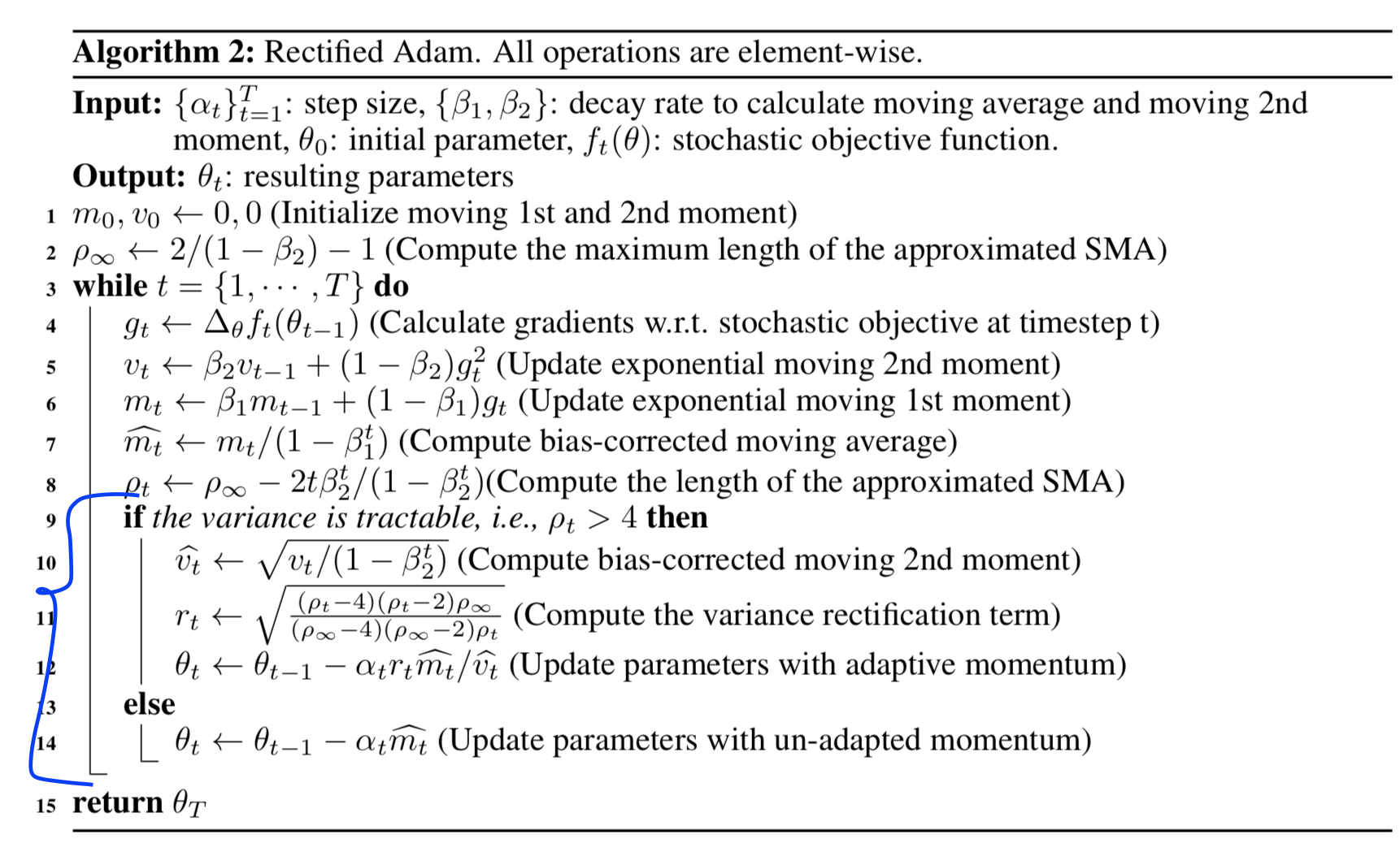
Adaptive learning has so far been very successful in benchmark datasets like CIFAR-10. However it comes with the pitfall of larger variance in the early stage of training. The authors of R-Adam suggests a warmup heuristic to tackle tis problem and works as a variance reduction technique.
To be more specific, Adaptive learning meathods have undesirably large variance in the early stage of model training since it uses limited amount of training samples. Hence to reduce this variance, it is better to use smaller learning rates in the first few epochs of training.
The authors suggest the following to rectify this.
- Use low learning rate as a warm up rate.
- During training, look for stabilization in variance, and increase learning rate and update paremeters using adaptive momentum.
Below is the changes to Adam known as R-Adam.

Training CIFAR-10 with R-Adam vs Adam
I trained a CIFAR-10 from scratch to look for the change in performance. The network is a 3 layer CNN with Relu as activations. I use the below optimizer setting.
# use optimizer based on input argument
if args["optimizer"] == "adam":
	print("Using Adam")
	opt = Adam(lr=1e-3)
else:
    print("Using Rectified-Adam")
    opt = RAdam(total_steps=5000, warmup_proportion=0.1, min_lr=1e-5)
A 3 layer CNN is modelled as below.
def define_model(opt = opt):
	model = Sequential()
	model.add(Conv2D(32, (3, 3), activation='relu', kernel_initializer='he_uniform', padding='same',input_shape=(32, 32, 3)))
	model.add(Conv2D(32, (3, 3), activation='relu', kernel_initializer='he_uniform', padding='same'))
	model.add(MaxPooling2D((2, 2)))
	model.add(Dropout(0.2))
	model.add(Conv2D(64, (3, 3), activation='relu', kernel_initializer='he_uniform', padding='same'))
	model.add(Conv2D(64, (3, 3), activation='relu', kernel_initializer='he_uniform', padding='same'))
	model.add(MaxPooling2D((2, 2)))
	model.add(Dropout(0.2))
	model.add(Conv2D(128, (3, 3), activation='relu', kernel_initializer='he_uniform', padding='same'))
	model.add(Conv2D(128, (3, 3), activation='relu', kernel_initializer='he_uniform', padding='same'))
	model.add(MaxPooling2D((2, 2)))
	model.add(Dropout(0.2))
	model.add(Flatten())
	model.add(Dense(128, activation='relu', kernel_initializer='he_uniform'))
	model.add(Dropout(0.2))
	model.add(Dense(10, activation='softmax'))

	model.compile(optimizer=opt, loss='categorical_crossentropy', metrics=['accuracy'])
	return model
Results
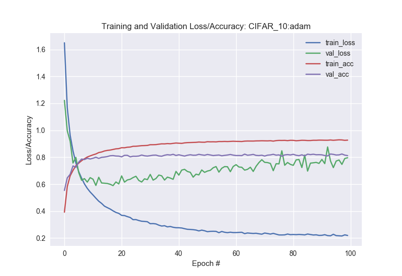
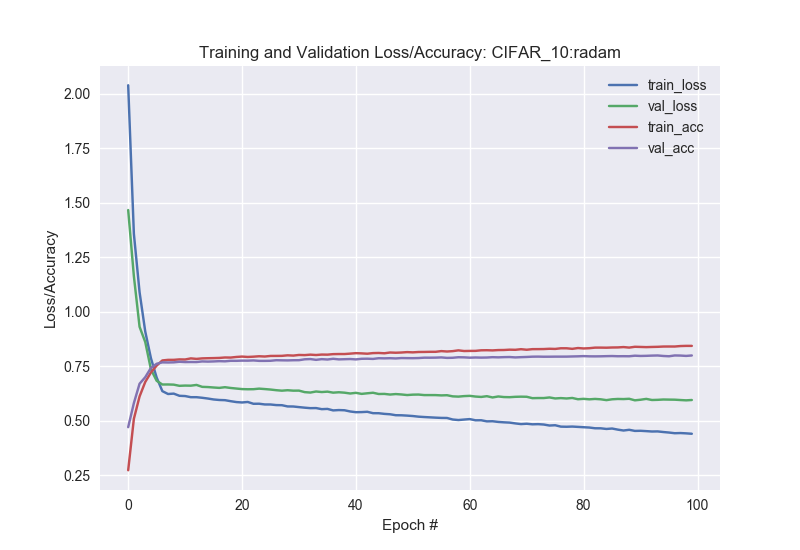
As we see, the training progress with R-Adam is a lot stable as compared to Adam.

We however see a a lower accuracy with R-Adam as compared to Adam, with all other parameter setting remaining constant.

The whole code for the project can be found at my GitHub.
Sources
[1] Ian Goodfellow-et-al-2016 “Deep Learning book”.
[2] Liyuan Liu ‘On the Variance of the Adaptive Learning Rate and Beyond’.
[3] Adrian Rosebrock ‘PyImageSearch’